13.4. XAFS: Post-edge Background Subtraction

Background subtraction is one of the most important data processing steps in EXAFS analysis, converting the measured \(\mu(E)\) into the \(\chi(k)\) ready for quantitative analysis. In Larch, this step is performed by the autobk() function, which has many options and subtleties. This section is devoted to background subtraction with the autobk() function and the underlying algorithm it uses.

13.4.1. The autobk() function

autobk(energy, mu=None, group=None, rbkg=1.0, ...)

Determine the post-edge background function, \(\mu_0(E)\), and corresponding \(\chi(k)\).

Parameters

• energy – 1-d array of x-ray energies, in eV

• mu – 1-d array of \(\mu(E)\)

• group – output group (and input group for e0 and edge_step).

• rbkg – distance (in \(\rm\AA\)) for \(\chi(R)\) above which the signal is ignored. Default = 1.

• e0 – edge energy, in eV. If None, it will be determined.

• edge_step – edge step. If None, it will be determined.

• pre_edge_kws – dictionary containing keyword arguments to pass to pre_edge().

• nknots – number of knots in spline. If None, it will be determined.

• kmin – minimum \(k\) value [0]

• kmax – maximum \(k\) value [None, full data range].

• kweight – \(k\) weight for FFT. [1]

• dk – FFT window window parameter. [0.1]

• win – FFT window function name. [‘hanning’]

• nfft – array size to use for FFT [2048]

• kstep – \(k\) step size to use for FFT [0.05]

• k_std – optional \(k\) array for standard \(\chi(k)\) [None]

• chi_std – optional \(\chi\) array for standard \(\chi(k)\) [None]

• nclamp – number of energy end-points for clamp [2]

• clamp_lo – weight of low-energy clamp [1]

• clamp_hi – weight of high-energy clamp [1]

• calc_uncertaintites – Flag to calculate uncertainties in \(\mu_0(E)\) and \(\chi(k)\) [True]

• err_sigma – sigma level for uncertainties in mu_0(E) and chi(k) [1]

Returns

None.

Follows the First Argument Group convention, using group members named energy and mu. The following data is put into the output group:

attribute	meaning
bkg	array of \(\mu_0(E)\) (not normalized)
chie	array of \(\chi(E)\) values.
k	array of \(k\) values, on uniform grid.
chi	array of \(\chi(k)\) values, the EXAFS.
delta_chi	array of uncertainty in \(\chi(k)\).
delta_bkg	array of uncertainty in \(\mu_0(E)\).
autobk_details	Group of arrays with autobk details.

Here, the arrays group.k, group.chi will be the same length, giving \(\chi(k)\) from 0 to a maximum k value set by kmax or the range of available data. The arrays group.bkg and group.chie will correspond to the input energy array.

The parameters e0 and edge_step are needed to determine \(\chi(k)\), and can be specified here. If they are not, but the input group has attributes e0 and edge_step – say, from running pre_edge() – those values will be used. If values cannot be found in either place, they will be determined by calling pre_edge() from within autobk(), and the output parameters from pre_edge() will be added to the output group here. The pre_edge_kws argument can be used here to hold a dictionary of parameters to pass to pre_edge().

If calc_uncertainties is set to True, the outputs group.delta_chi and group.delta_bkg, holding the uncertainties in \(\chi(k)\) and \(\mu_0(E)\), respectively. These calculations are relatively costly, and can take 20 times longer to determine \(\chi(k)\) and \(\mu_0(E)\) themselves.

The group.autobk_details group will contain the following attributes:

attribute	meaning
spline_pars	Parameters used for determining \(\mu_0(E)\) spline.
init_bkg	Initial value for \(\mu_0(E)\)
init_chi	Initial value for \(\chi(k)\)
knots_e	Spline knot energies
knots_y	Spline knot values
init_knots_y	Initial Spline knot values

13.4.2. The AUTOBK Algorithm

The background subtraction method used is the AUTOBK algorithm (see [Newville et al. (1993)]), in which a spline function is matched to the low-R components of the resulting \(\chi(k)\).

For reference, \(k = \sqrt{2m_e (E-E_0)/\hbar^2}\) is the wavenumber of the ejected photo-electron, where \(E_0\) is the absorption threshold energy (the 0 of photo-electron energy). For \(k\) in units of \(\rm \AA^{-1}\) and \(E\) in units of eV, \(k \approx \sqrt{(E-E_0)/3.81}\). With this conversion of energy to wavenumber, \(\chi(k)\) is defined from

\(\chi(E) = \frac{\mu(E)-\mu_0(E)}{\Delta\mu}\)

where \(\mu_0(E)\) represents the idealized x-ray absorption of a bare atom, embedded in the molecular or solid environment, but without scattering of the outgoing photo-electron that gives rise to the EXAFS, and \(\Delta\mu\) is the edge step in \(\mu(E)\).

The quantity \(\mu_0(E)\) cannot be independently measured. Instead, we empirically determine it here given the dxta for \(\mu(E)\) by fitting a spline (a piece-polynomial function that is easily adjusted even while its smoothness is controlled) to \(\mu(E)\). An advantage to what could easily be described as an ad hoc approach is that the data for \(\mu(E)\) can include many systematic drifts and dependencies that are slowly varying with energy.

The definition above normalizes to the edge step \(\Delta\mu\) (edge_step) instead of the energy-dependent \(\mu_0(E)\), as is often described in introductory texts on EXAFS. The reason for this is essentially the same – so that we do not need to carefully take care of slow energy drifts in the measured \(\mu(E)\) or worry about having an absolute measure of \(\mu(E)\).

13.4.2.1. \(R_{\rm bkg}\) and spline for \(\mu_0(E)\)

A spline is a general mathematical function, and so using one to match \(\mu(E)\) that we will subtract from the same \(\mu(E)\) could easily match too well, and erase much of the data we’re interested in. Therefore, we have to carefully consider two aspects:

1. what portions of the spectrum we want it to match, and

2. how flexible the spline can be.

What we want is a \(\mu_0(E)\) that removes the low frequency (low-R) portions of the \(\chi\) spectra, and recognizing this can tell us how to determine both of these.

First, since we know the EXAFS oscillations do not extend far below the near-neighbor distance and since atoms are essentially never closer than 1 \(\rm\AA\), and generally more like 2 \(\rm\AA\), we can say that we want to remove the frequencies of \(\chi\) below some distance, \(R_{\rm bkg}\) (rbkg). That is, we want the spline function to be adjusted so that the components of \(\chi(R)\) below \(R_{\rm bkg}\) are minimized. We can use a default of 1 \(\rm\AA\), and recommend that the value be roughly half the expected near-neighbor distance.

To do this, we create a spline function consisting of \(N_{\rm knots}\) adjustable points (knots in the spline, where the second derivatives are allowed to change), evenly spaced in \(k\) (that is, quadratic in energy). We do a fit that adjusts the values of the function at each knot, computes \(\mu_0(E)\) by simple spline interpolation, calculates \(\chi(k)\), does a Fourier transform to \(\chi(R)\), and then seeks to minimize the components of \(\chi(R)\) below \(R_{\rm bkg}\).

This leads to the second question of how flexible to make the spline is answered from basic signal processing through the Nyquist-Shannon sampling theorem, which tells us how many adjustable parameters to use for our spline:

\[N_{\rm knots} = 1 + \frac{2R_{\rm bkg} \Delta k}{\pi}\]

where \(\Delta k\) is the \(k\) range of the data. This value can be over-ridden by specifing nknots, but this is strongly recommended against.

In this way we satisfy both considerations above: limiting the number of knots prevents the spline from being able to follow the frequencies of \(\chi(k)\) we care about most, and limiting the portion of the spectrum to be minimized to the very low-\(R\) components, we do not even try to match those frequencies. Thus, we are ensured of a \(\mu_0(E)\) that only removes the low-\(R\) components of \(\chi\).

13.4.2.2. Selecting Fourier transform parameters

In order to determine \(\mu_0(E)\), we must do a Fourier transform. These are discussed in more detail in the next section, but here we give the parameters affecting the Fourier transform used, and their default values.

argument	meaning	default, recommended values
kmin	\(k_{\rm min}\)	should be below 1.0
kmax	\(k_{\rm max}\)	highest \(k\) value. Useful data range.
kweight	\(kw\)	should be 0 or 1 (but not > 2)
win	window function name	Hanning, Parzen works well too.
dk	window sill size	should be 0 or 1
nfft	FFT array size	No reason to change this.
kstep	\(k\) step size	0.05. No reason to change this.

The most important point is that the Fourier transform used to fit and visualize \(\chi(k)\) is not necessarily the one to use here. In particular, the kweight parameter should be 0 or 1 here, as we want to emphasize the low-\(k\) portion of \(\chi(k)\). The default parameter values for autobk() are generally sufficient, and need only minor adjustments except in unusual cases.

13.4.2.3. Using a standard \(\chi(k)\)

We said above that we want to minimize the low-\(R\) components of \(\chi\). In principle, there should be some leakage of the first shell to fairly low-\(R\). This is especially noticeable for a short ligand (say, below 1.75 \(\rm\AA\) or so) of a low-Z atom (notably, C, N, and O). Normally, this is not a serious problem, but it does point out that \(\mu_0(E)\) might want to leave some first-shell leakage at low-\(R\).

To accout for this, you can proved a spectrum of \(\chi(k)\) for a standard that is meant to be close to the spectrum being analyzed. This is done by providing 2 arrays: k_std and chi_std, which need to be the same lenth. By providing these, the best values for \(\mu_0(E)\) will be those that minimize the Fourier transorm of the difference of \(\chi(k)\) for the data and standard. This can be especially helpful to give more consistent background for a set of related spectra.

13.4.2.4. End-point clamps for the spline

Because the spline is chosen to match the low-\(R\) components of \(\chi\), the process does not even look at how the resulting \(\mu_0(E)\) looks. This can lead to some unstable behavior at the end-points of the spline, causing \(\chi(k)\) to diverge at the ends.

This can be remedied by adding clamps to the end-points of \(chi(k)\) to the fit. That is, a few points at the low- and high-ends of the \(\chi(k)\) array are appended to the array to be minimized in the fit, which has the tendency to push the end-points of \(\chi(k)\) to zero.

There are three parameters influencing these end-points clamps. nclamp sets the number of data points of \(\chi(k)\) at the beginning and end of the \(k\) range to add to the fit. clamp_lo sets the weighting factor applied to the first nclamp points for the low-\(k\) end fo the data range, and clamp_hi sets the weighting factor applied to the last nclamp points at the high-\(k\) end.

There is not an easy way to determine ahead of time what the clamp parameters will be. Typically, nclamp need only be 1 to 5 data points (with 2 being the default). Setting nclamp to 0 will remove the clamps completely. Values for clamp_lo and clamp_hi are floating point numbers, and should range from about 1 (the default) to 10 or 20 for a very strong clamp that will almost certainly force \(\chi(k)\) to be 0 at the end-points.

13.4.2.5. Recommendations

Here, we give a few recommendations on what parameters most affect the background subtraction. These parameters are (in roughly increasing order):

0. rbkg: This is the main parameter that sets how flaexible the spline function can be.

1. e0: It can be hard to know what \(E_0\) should be for any XAFS spectra. As this sets the value of \(k=0\), it will affect the location of the knots, and can have a profound affect on the results. If you’re unhappy with the \(\mu_0(E)\) and \(\chi(k)\), playing with the e0 parameter.

2. kweight: Increasing this emphasizes the fit at high k. Trying both values of 0 and 1 is always a good idea.

3. clamp_lo and clamp_hi: If \(\mu_0(E)\) swoops up or down at the endpoints too much, increasing these values can help greatly.

13.4.3. Examples

Here, we give a few examples using autobk(), and outline some of its features.

13.4.3.1. Basic example

The simplest example of reading data and doing background subtraction would using all the default inputs would be:

## examples/xafs/doc_autobk1.lar

fname = '../xafsdata/cu_rt01.xmu'
cu = read_ascii(fname)
autobk(cu.energy, cu.mu, rbkg=1.0, group=cu)

plot_bkg(cu, emin=-100, emax=400)

plot_chik(cu, kweight=1, win=2)
## end of examples/xafs/doc_autobk1.lar

with the resulting outputs looking like this:

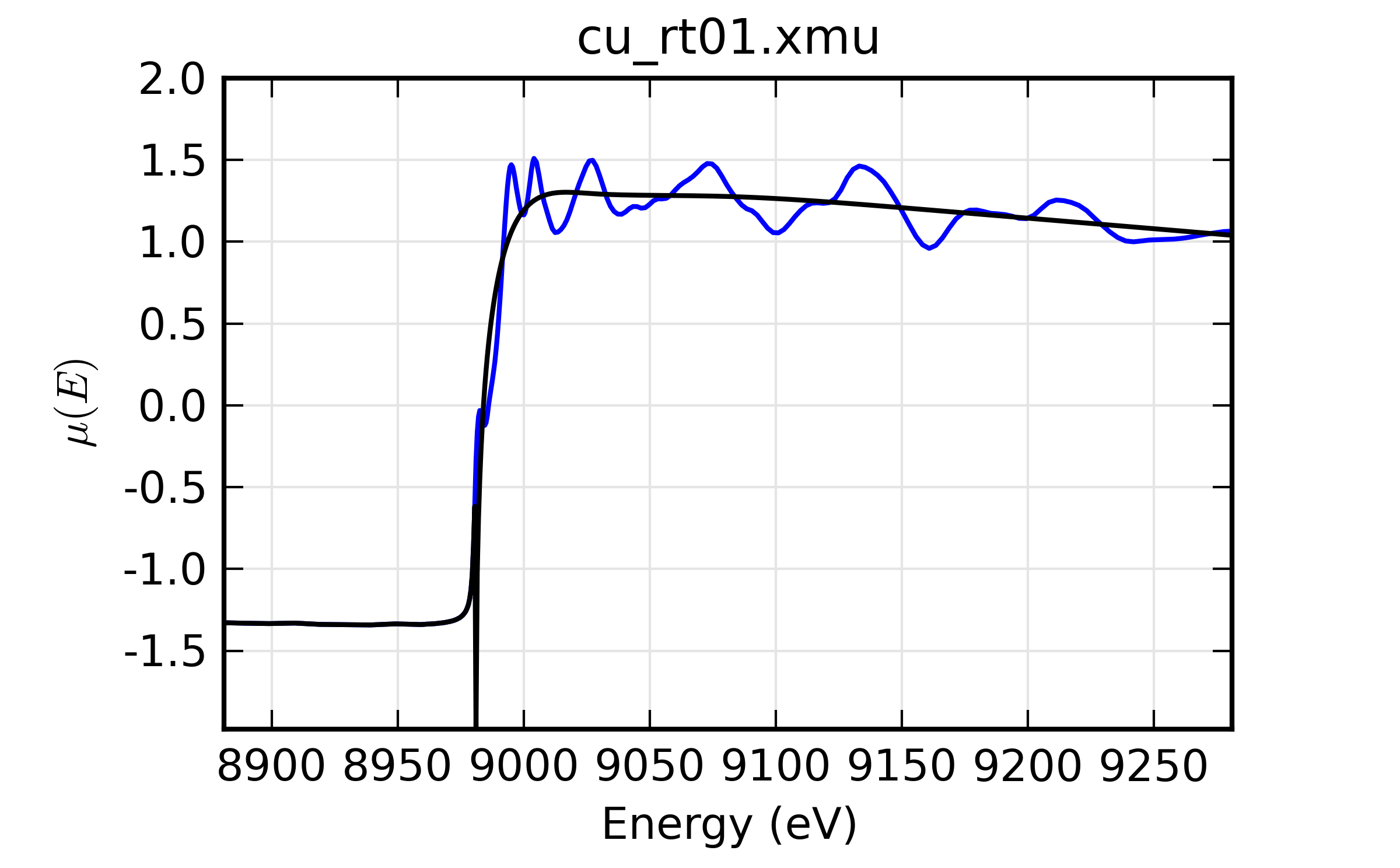
Figure 13.4.3.1 \(\mu(E)\) and background \(\mu_0(E)\)

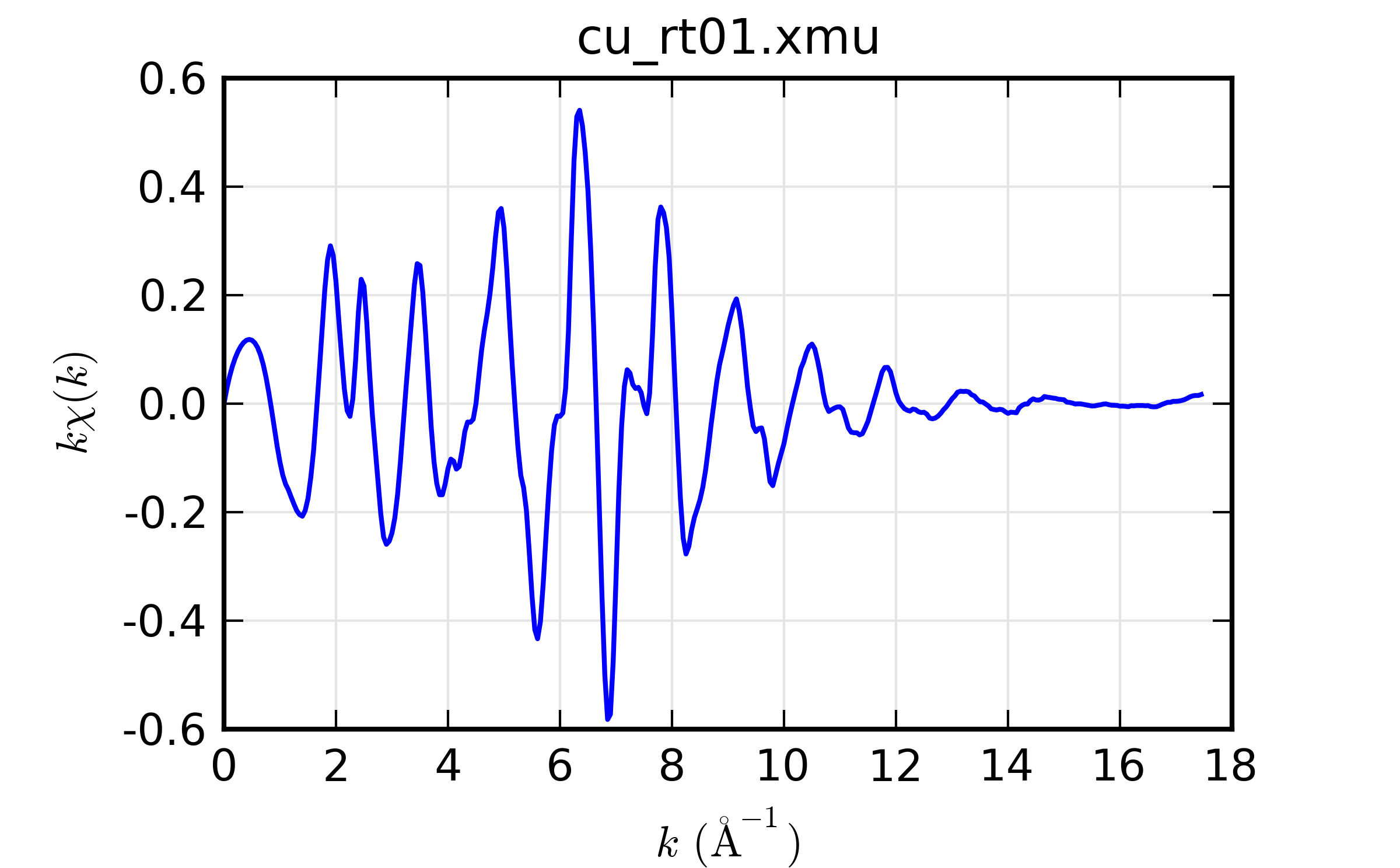
Figure 13.4.3.2 resulting \(k\chi(k)\)

Example of simple usage of autobk() for Cu metal.

Thus demonstrating that we can process data on Cu metal.

For a slightly more challenging example, we try the As K-edge of scorodite (\(\rm FeAsO4 \cdot (nH_2O)\)). Here, we start by reading in data and constructing \(\mu(E)\), then run autobk(). We take most of the default values for pararmeters, but pass explicit parameters such as nnorm to pre_edge() using pre_edge_kws. Setting these parameters is not critically important for this data set, and is mostly here to demonstrate the method for passing arguments to pre_edge().

## examples/xafs/doc_autobk2.lar

fname = '../xafsdata/scorodite_as_xafs.001'
title = 'FeAsSO4  (scorodite)'
dat = read_ascii(fname)
dat.mu = ln(dat.i0/dat.i1)

autobk(dat.energy, dat.mu, rbkg=1.0, group=dat)
plot_bkg(dat, emin=-150)
plot_chik(dat, kweight=2, win=2)

## end of examples/xafs/doc_autobk2.lar

The resulting outputs looks OK:

Example usage of autobk() for \(\rm FeAsO4 \cdot (nH_2O)\).

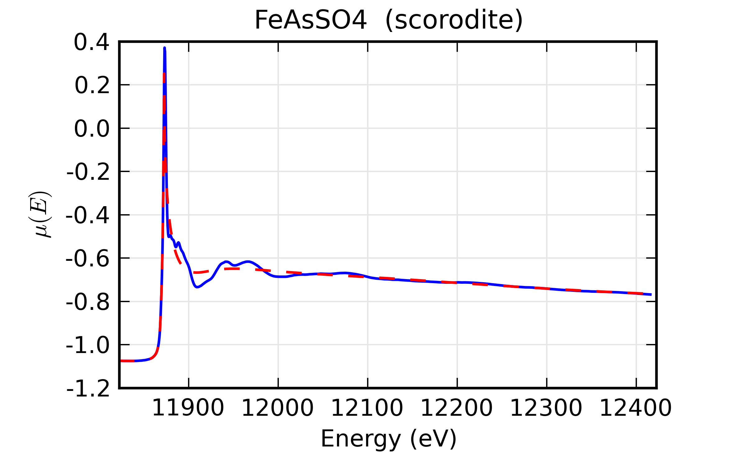
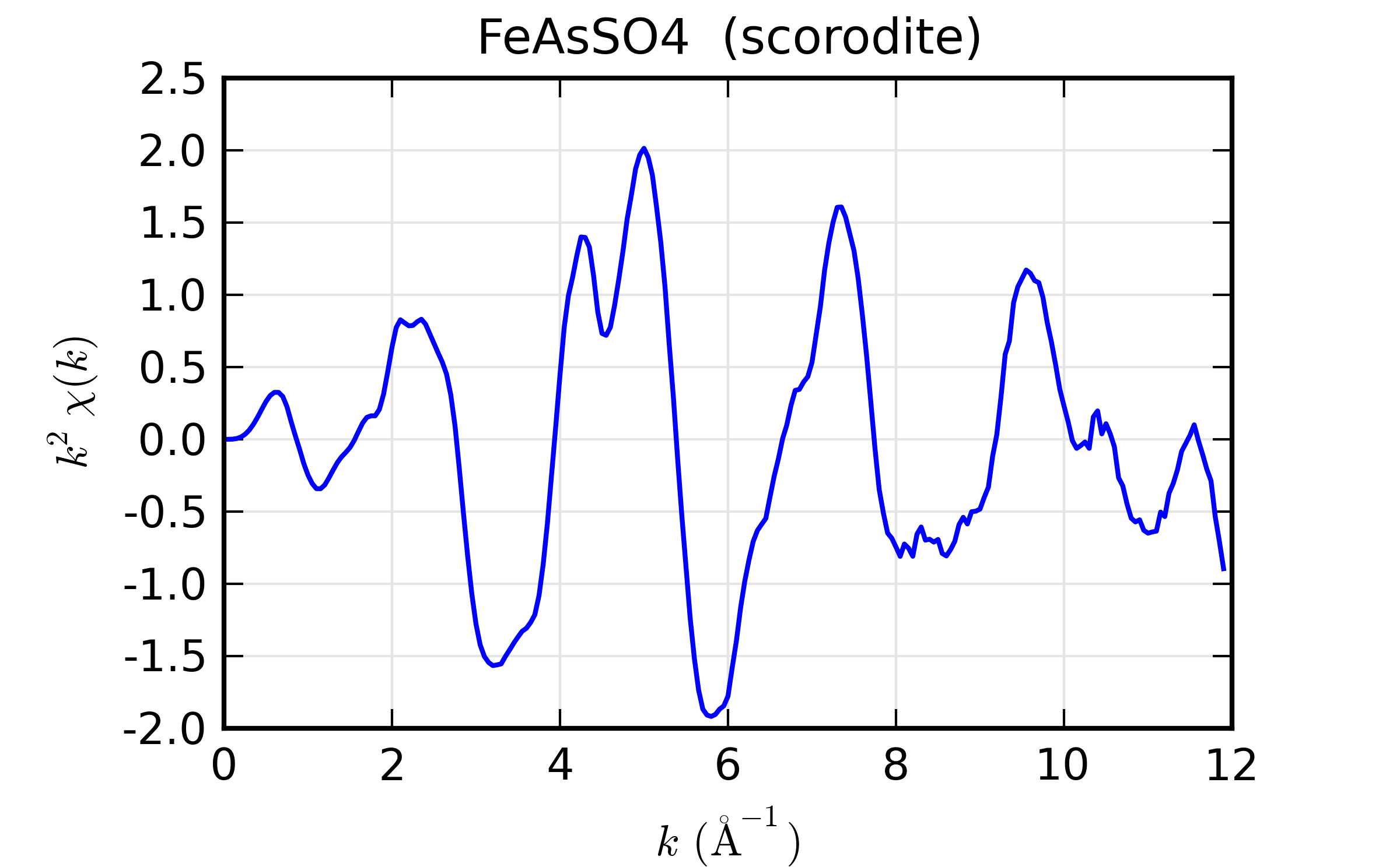
A close examimation of \(k^2\chi(k)\) suggests we might be able to do better, which brings us to the next section.

13.4.3.2. Adjusting spline clamps

For the scorodite example above, the XAFS diverges from 0 at the high-\(k\) end of the spectra. Playing with the spline clamps discussed above, we try a few options to study the effect of adding a clamp:

## examples/xafs/doc_autobk3.lar
fname = '../xafsdata/scorodite_as_xafs.001'
title = 'FeAsSO4  (scorodite)'
dat = read_ascii(fname)
dat.mu    = ln(dat.i0/dat.i1)

autobk(dat.energy, dat.mu, rbkg=1.0, group=dat, clamp_hi=0)
dat.chi0 = dat.chi * dat.k**2
dat.bkg0 = dat.bkg

autobk(dat.energy, dat.mu, rbkg=1.0, group=dat, clamp_hi=10)
dat.chi10 = dat.chi * dat.k**2
dat.bkg10 = dat.bkg

autobk(dat.energy, dat.mu, rbkg=1.0, group=dat, clamp_hi=50)
dat.chi50 = dat.chi * dat.k**2
dat.bkg50 = dat.bkg

newplot(dat.k, dat.chi0, label='clamp_hi=0', show_legend=True,
        xlabel=r'$k \rm\, (\AA^{-1})$',  ylabel=r'$k^2\chi(k)$',
        title='Effect of clamp_hi')

plot(dat.k, dat.chi10, label='clamp_hi=10', show_legend=True)
plot(dat.k, dat.chi50, label='clamp_hi=50', show_legend=True)

## end of examples/xafs/doc_autobk3.lar

results in the following comparison:

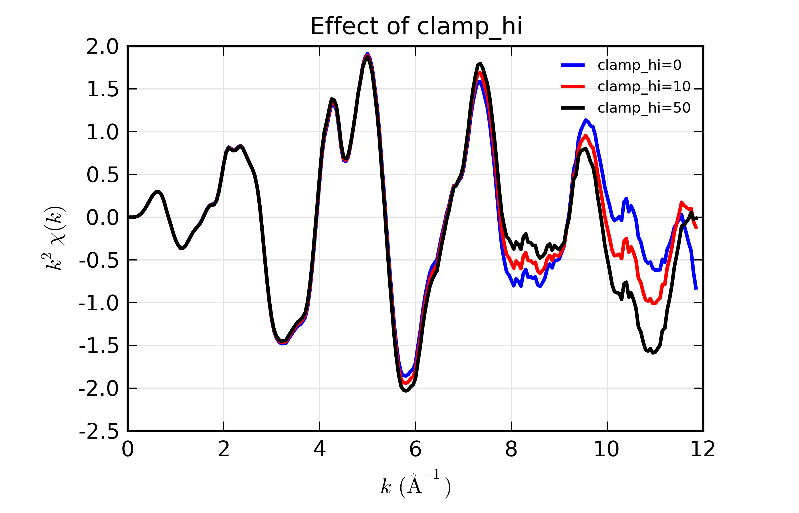
Figure 13.4.3.3 Influence of spline clamps of \(\chi(k)\)

13.4.3.3. Using a Standard \(\chi(k)\)

Since the EXAFS contribution from the first shell is not perfectly isolated in \(R\), it can leak into portion of \(\chi(R)\) below \(R_{\rm bkg}\). It may be desirable to not simply reduce the portion of \(\chi(R)\) below \(R_{\rm bkg}\), but to account for the expected leakage from the first shell. To do this, you can provide a standard \(\chi(k)\) spectrum that will simulate the first shell by specify arrays for k_std and chi_std arrays to the autobk() function.

As an example:

## examples/xafs/doc_autobk4.lar

fname = '../xafsdata/cu.xmu'
chi_fname = '../xafsdata/cu10k.chi'

cu1 = read_ascii(fname)

chidat = read_ascii(chi_fname, labels='k chi')

pre_edge(cu1.energy, cu1.mu, group=cu1)

cu2 = copy(cu1)

autobk(cu1.energy, cu1.mu, rbkg=1, group=cu1)

# now with std...
autobk(cu2.energy, cu2.mu, rbkg=1, group=cu2, k_std=chidat.k, chi_std=chidat.chi)

plot_chik(cu1, kweight=2, label='no std')
plot_chik(cu2, kweight=2, label='with std', new=False)
## end of examples/xafs/doc_autobk4.lar

References

Newville et al. (1993)

M. Newville, P. Livins, Y. Yacoby, J. J. Rehr, and E. A. Stern. Near-edge x-ray-absorption fine structure of Pb: A comparison of theory and experiment. Physical Review B, 47(21):14126–14131, 1993. doi:10.1103/PhysRevB.47.14126.